Multiview Neural Surface Reconstruction by Disentangling Geometry and Appearance#

  • Authors: Lior Yariv, Yoni Kasten, Dror Moran, Meirav Galun, Matan Atzmon, Ronen Basri, Yaron Lipman

  • Affiliations: Weizmann Institute of Science

  • NeurIPS 2020

  • Links: arXiv, Project Page, Code

Summary#

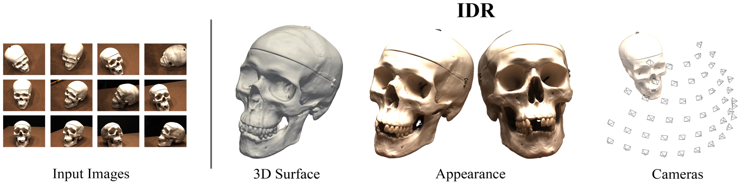
In this work the authors introduce a neural network architecture that simultaneously learns the unknown geometry, camera parameters, and a neural renderer that approximates the light reflected from the surface towards the camera. By training the network on real world 2D images of objects with different material properties, lighting conditions, and noisy camera initializations from the DTU MVS dataset, the model can produce state-of-the-art 3D surface reconstructions with high fidelity, resolution, and detail.

../_images/fig-022.png

Key Ideas#

The goal is to reconstruct the geometry of an object from masked 2D images with possibly rough or noisy camera information. There are three unknowns:

  • geometry \(\theta \in \mathbb{R}^m\)

  • appearance \(\gamma \in \mathbb{R}^n\)

  • cameras \(\tau \in \mathbb{R}^k\)

../_images/fig-012.png

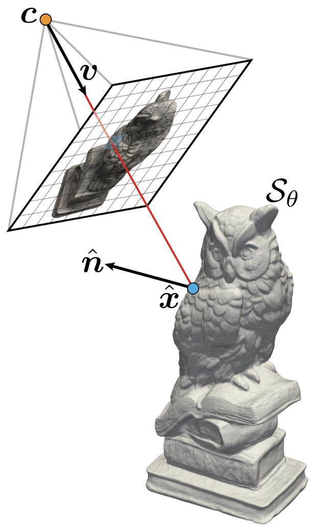
The geometry is represented as the zero level set of an MLP \(f\)

\[S_\theta = \{ \boldsymbol{x} \in \mathbb{R}^3 \mid f(\boldsymbol{x}; \theta) = 0\}\]

IDR forward model. Let the pixel be \(p\) and the ray through pixel \(p\) be \(R_p(\tau) = \{c_p + tv_p \mid t \geq 0\}\). Let \(\hat{\boldsymbol{x}}_p = \hat{\boldsymbol{x}}_p(\theta, \tau)\) denote the first intersection. The rendered color of the pixel \(L_p\) is given by

\[L_p(\theta, \gamma, \tau) = M(\hat{\boldsymbol{x}}_p, \hat{\boldsymbol{n}}_p, \hat{\boldsymbol{z}}_p, \boldsymbol{v}_p; \gamma)\]

Approximation of the surface light field. The surface light field radiance \(L\) is determined by two functions: the bidrectional reflectance distribution function (BRDF) and the light emitted in the scene.

  • The BRDF function \(B(\boldsymbol{x}, \boldsymbol{n}, \boldsymbol{w}^o, \boldsymbol{w}^i)\) describes the proportion of reflected radiance leaving the surface point \(\boldsymbol{x}\) with normal \(\boldsymbol{n}\) at direction \(\boldsymbol{w}^o\) with respect to the incoming radiance from direction \(\boldsymbol{w}^i\).

  • The light sources are described by a function \(L^e(\boldsymbol{x}, \boldsymbol{w}^o)\) measuring the emitted radiance of light at point \(\boldsymbol{x}\) in direction \(\boldsymbol{w}^o\).

The overall rendering equation is given by

\[L(\hat{\boldsymbol{x}}, \boldsymbol{w}^o) = L^e(\hat{\boldsymbol{x}}, \boldsymbol{w}^o) + \int_\Omega B(\hat{\boldsymbol{x}}, \hat{\boldsymbol{n}}, \boldsymbol{w}^i, \boldsymbol{w}^o)L^i(\hat{\boldsymbol{x}}, \boldsymbol{w}^i) d \boldsymbol{w}^i = M(\hat{\boldsymbol{x}}, \hat{\boldsymbol{n}}, \boldsymbol{v}; \gamma)\]

where \(M\) is a sufficiently large MLP approximating \(M_0\). For \(M\) to be able to represent the correct light reflected from a surface point \(\boldsymbol{x}\) , i.e., be \(\mathcal{P}\) -universal, it has to receive as arguments also \(\boldsymbol{v}, \boldsymbol{n}\) .

Masked rendering. Consider the indicator function identifying whether a certain pixel is occupied by the rendered object

\[S(\theta, \tau) = \mathrm{sigmoid} \left( - \alpha \min_{t \geq 0} f(c + tv; \theta) \right)\]

which approximates \(S(\theta, \tau)\) as \(\alpha \to \infty\).

Loss. The loss is given by

\[\begin{split}\mathcal{L}(\theta, \gamma, \tau) & = \mathcal{L}_\text{RGB}(\theta, \gamma, \tau) + \rho \mathcal{L}_\text{mask}(\theta, \tau) + \lambda \mathcal{L}_\text{E}(\theta) \\ \mathcal{L}_\text{RGB}(\theta, \gamma, \tau) & = \frac{1}{\lvert P \rvert} \sum_{p \in P^\text{in}} \lvert I_p - L_p(\theta, \gamma, \tau) \\ \mathcal{L}_\text{mask}(\theta, \tau) & = \frac{1}{\alpha \lvert P \rvert} \sum_{\alpha \lvert P \rvert} \text{CE}(O_p, S_{p, \alpha}(\theta, \tau)) \\ \mathcal{L}_\text{E}(\theta) & = \mathbb{E}_x( \lVert \nabla_x f(x; \theta) \rVert - 1)^2\end{split}\]

where \(\mathcal{L}_\text{E}\) is the Implicit Geometric Regularization (IGR) incorporating the Eikonal regularization [1].

Technical Details#

Notes#

References#

[1] A. Gropp, L. Yariv, N. Haim, M. Atzmon, Y. Lipman. Implicit geometric regularization for learning shape. In arXiv, 2020.